library(data.table)
library(ggplot2)
library(ggpubr)
library(ggrepel)
library(genepi.utils)
library(tibble)
library(knitr)Tissue-partitioned BMI instrument procedure
Motivation
What does the weighting by PPH4 do to tissue partitioned BMI instruments? Let’s simulate some tissue partitioned BMI MR results.
BMI data
First load the BMI GWAS.
bmi    <- readRDS(file.path(TPMR_DIR, "output", "tmp_objects", "obj_bmi.RDS"))
clumps <- clump(as.data.table(bmi), p1=5e-8, r2=0.001, kb=10000, plink2=PLINK2, plink_ref=UKBB_REFERENCE)[index==TRUE]
bmi    <- subset_gwas(bmi, clumps$rsid)
kable(head(clumps, 5), caption = "BMI lead variants")| rsid | chr | bp | ea | oa | eaf | beta | se | p | n | ncase | trait | id | strand | imputed | info | q | q_p | i2 | proxy_rsid | proxy_chr | proxy_bp | proxy_ea | proxy_oa | proxy_eaf | proxy_r2 | snp | index | clump |
|---|---|---|---|---|---|---|---|---|---|---|---|---|---|---|---|---|---|---|---|---|---|---|---|---|---|---|---|---|
| rs10007906 | 4 | 31023610 | A | C | 0.360300 | 0.0133000 | 0.0018000 | 0 | 686479 | NA | bmi | combined_bmi_giant_ukb_annot.txt | NA | NA | NA | NA | NA | NA | NA | NA | NA | NA | NA | NA | NA | rs10007906 | TRUE | 291 |
| rs1000940 | 17 | 5283252 | A | G | 0.701300 | -0.0154000 | 0.0018000 | 0 | 794558 | NA | bmi | combined_bmi_giant_ukb_annot.txt | NA | NA | NA | NA | NA | NA | NA | NA | NA | NA | NA | NA | NA | rs1000940 | TRUE | 142 |
| rs1007934 | 14 | 73463479 | A | G | 0.415000 | -0.0120000 | 0.0017000 | 0 | 692411 | NA | bmi | combined_bmi_giant_ukb_annot.txt | NA | NA | NA | NA | NA | NA | NA | NA | NA | NA | NA | NA | NA | rs1007934 | TRUE | 407 |
| rs10125137 | 9 | 118644190 | T | C | 0.641786 | -0.0117273 | 0.0020523 | 0 | 463005 | NA | bmi | combined_bmi_giant_ukb_annot.txt | NA | NA | NA | NA | NA | NA | NA | NA | NA | NA | NA | NA | NA | rs10125137 | TRUE | 811 |
| rs10131890 | 14 | 97258752 | A | C | 0.950300 | -0.0222000 | 0.0039000 | 0 | 691777 | NA | bmi | combined_bmi_giant_ukb_annot.txt | NA | NA | NA | NA | NA | NA | NA | NA | NA | NA | NA | NA | NA | rs10131890 | TRUE | 846 |
Heart failure data
Load the heart failure GWAS.
hf <- readRDS(file.path(TPMR_DIR, "output", "tmp_objects", "obj_hf_allcause.RDS"))
hf <- subset_gwas(hf, clumps$rsid)
Harmonise the datasets
h <- MR(bmi, hf)
kable(head(as.data.table(h),5), caption = "Harmonised BMI:HF dataset")| rsid | chr | bp | ea | oa | bx | bxse | px | by | byse | py | proxy_e_snp | proxy_o_snp | index_snp | group | ld_info | exposure | outcome |
|---|---|---|---|---|---|---|---|---|---|---|---|---|---|---|---|---|---|
| rs10007906_C_A | 4 | 31023610 | A | C | 0.0133000 | 0.0018000 | 0 | 0.0039 | 0.0051 | 0.44980 | NA | NA | TRUE | NA | FALSE | bmi | hf_allcause |
| rs1000940_G_A | 17 | 5283252 | A | G | -0.0154000 | 0.0018000 | 0 | 0.0011 | 0.0050 | 0.82970 | NA | NA | TRUE | NA | FALSE | bmi | hf_allcause |
| rs1007934_G_A | 14 | 73463479 | A | G | -0.0120000 | 0.0017000 | 0 | -0.0092 | 0.0049 | 0.05931 | NA | NA | TRUE | NA | FALSE | bmi | hf_allcause |
| rs10125137_C_T | 9 | 118644190 | T | C | -0.0117273 | 0.0020523 | 0 | 0.0033 | 0.0049 | 0.50820 | NA | NA | TRUE | NA | FALSE | bmi | hf_allcause |
| rs10131890_C_A | 14 | 97258752 | A | C | -0.0222000 | 0.0039000 | 0 | -0.0211 | 0.0099 | 0.03310 | NA | NA | TRUE | NA | FALSE | bmi | hf_allcause |
Run the MR
This is just the plain MR of BMI on HF.
res <- run_mr(h)
kable(res, caption = "BMI:HF Mendelian randomisation")| method | correlation | exposure | outcome | n_snp | b | b_se | p | intercept | int_se | int_p | qstat | qstat_p | fstat | condfstat | overdispersion | n_pc | n_hunted | slopehunter_pi | slopehunter_ent |
|---|---|---|---|---|---|---|---|---|---|---|---|---|---|---|---|---|---|---|---|
| mr_ivw | FALSE | bmi | hf_allcause | 874 | 0.4872820 | 0.0165599 | 0 | 0.0000000 | NA | NA | 1592.460 | 0 | 60.70091 | NA | NA | NA | NA | NA | NA |
| mr_egger | FALSE | bmi | hf_allcause | 874 | 0.5367727 | 0.0464790 | 0 | -0.0008232 | 0.0007224 | 0.2544728 | 1590.092 | 0 | NA | NA | NA | NA | NA | NA | NA |
| mr_weighted_median | FALSE | bmi | hf_allcause | 874 | 0.5078217 | 0.0236696 | 0 | 0.0000000 | NA | NA | NA | NA | NA | NA | NA | NA | NA | NA | NA |
| mr_weighted_mode | FALSE | bmi | hf_allcause | 874 | 0.5456300 | 0.0523114 | 0 | 0.0000000 | NA | NA | NA | NA | NA | NA | NA | NA | NA | NA | NA |
Plot MR
Plot MR result of BMI on HF.
plot_mr(h, res)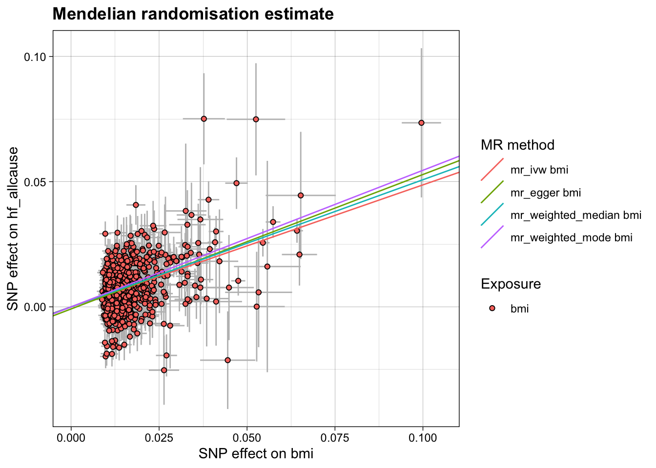
Select variants - MR with a subset of BMI variants
In the Leyden et al. 2022 paper 86 variant colocalise with adipose tissue eQTLs and 140 colocalise with brain tissue eQTLs. There is overlap between the two tissues of 43 variants. Let’s run the run of BMI on HF just using these variants - just looks like a similar version of the previous plot but with fewer points.
set.seed(123)
tissue1_varid <- sample(h@snps, 140)
overlap_varid <- sample(tissue1_varid, 43)
tissue2_varid <- c(overlap_varid, sample(h@snps[!h@snps %in% overlap_varid], 86-43))

# turn of variants not in either tissue
h@index_snp[!h@snps %in% c(tissue1_varid, tissue2_varid)] <- FALSE
h@exposure <- "BMI tissue 1/2 SNPs"

res1 <- run_mr(h)
kable(res1, caption = "BMI:HF Mendelian randomisation (Tissue 1 & 2 SNPs only)")| method | correlation | exposure | outcome | n_snp | b | b_se | p | intercept | int_se | int_p | qstat | qstat_p | fstat | condfstat | overdispersion | n_pc | n_hunted | slopehunter_pi | slopehunter_ent |
|---|---|---|---|---|---|---|---|---|---|---|---|---|---|---|---|---|---|---|---|
| mr_ivw | FALSE | BMI tissue 1/2 SNPs | hf_allcause | 177 | 0.5108471 | 0.0363407 | 0e+00 | 0.0000000 | NA | NA | 304.2402 | 0 | 61.28134 | NA | NA | NA | NA | NA | NA |
| mr_egger | FALSE | BMI tissue 1/2 SNPs | hf_allcause | 177 | 0.5475313 | 0.1037260 | 1e-07 | -0.0006034 | 0.0015974 | 0.7056336 | 303.9924 | 0 | NA | NA | NA | NA | NA | NA | NA |
| mr_weighted_median | FALSE | BMI tissue 1/2 SNPs | hf_allcause | 177 | 0.5730810 | 0.0494983 | 0e+00 | 0.0000000 | NA | NA | NA | NA | NA | NA | NA | NA | NA | NA | NA |
| mr_weighted_mode | FALSE | BMI tissue 1/2 SNPs | hf_allcause | 177 | 0.5887868 | 0.1022882 | 0e+00 | 0.0000000 | NA | NA | NA | NA | NA | NA | NA | NA | NA | NA | NA |
plot_mr(h, res1)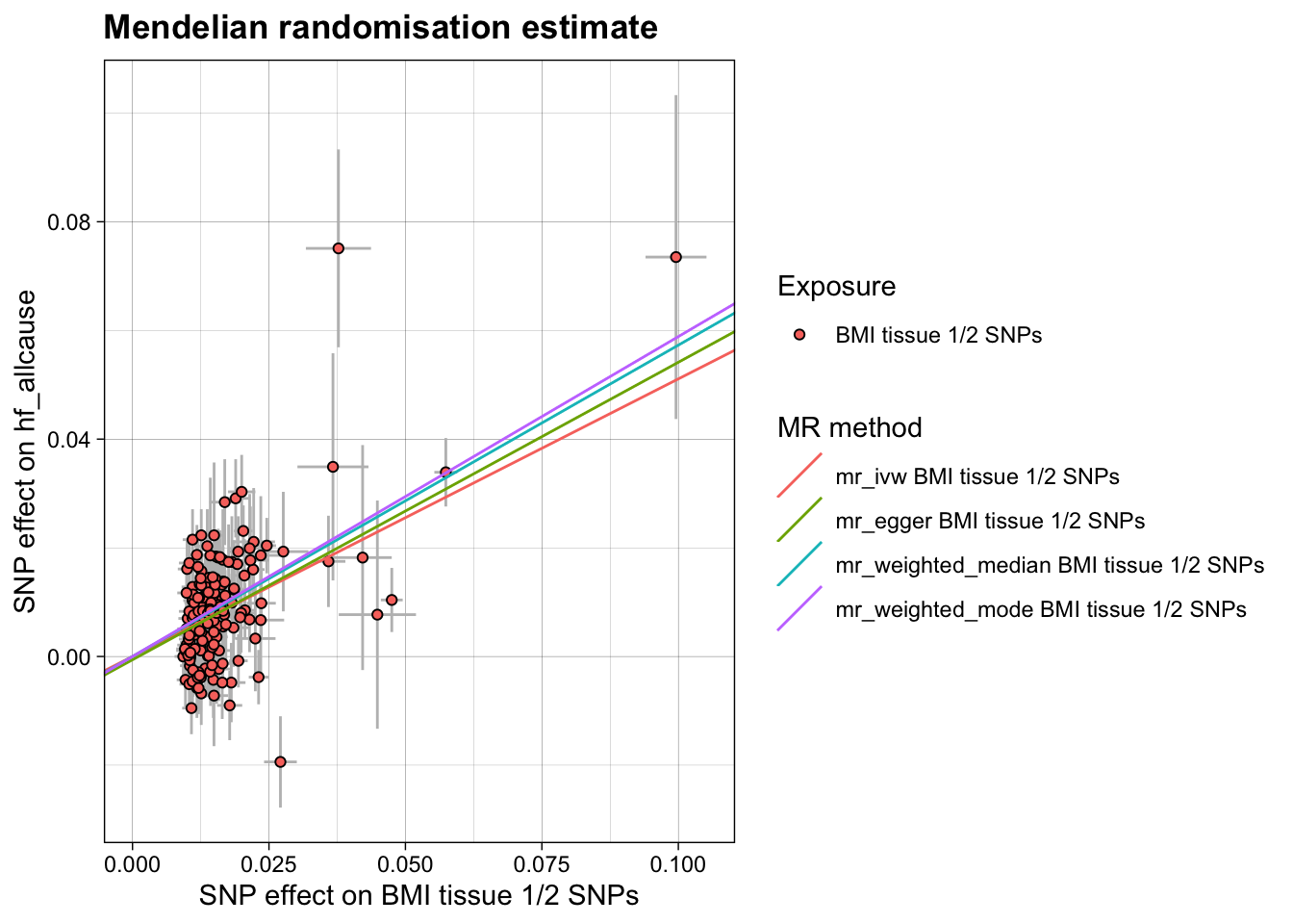
Run multivariable MR (unweighted)
Now lets turn this into a multivariable MR situation, with BMI variants for tissues one and BMI variants for tissue 2, against HF. The results are the same, as expected, because there is no differential weighting of the betas, effectively they are just the same instrument. So far nothing new.
# copy of BMI for tissue 1
bmi_t1 <- bmi
bmi_t1@id <- "bmi tissue 1"
bmi_t1@trait <- "bmi tissue 1"

# copy of BMI for tissue 2
bmi_t2 <- bmi
bmi_t2@id <- "bmi tissue 2"
bmi_t2@trait <- "bmi tissue 2"

# harmonise
h_mvmr <- MR(list(bmi_t1, bmi_t2), hf)

# turn of variants not in either tissue
h_mvmr@index_snp[!h_mvmr@snps %in% c(tissue1_varid, tissue2_varid)] <- FALSE

res2 <- run_mr(h_mvmr, methods="mr_ivw")
kable(res2, caption = "BMI:HF MV Mendelian randomisation")| method | correlation | exposure | outcome | n_snp | b | b_se | p | intercept | int_se | int_p | qstat | qstat_p | fstat | condfstat | overdispersion | n_pc | n_hunted | slopehunter_pi | slopehunter_ent |
|---|---|---|---|---|---|---|---|---|---|---|---|---|---|---|---|---|---|---|---|
| mr_mvivw | FALSE | bmi tissue 1 | hf_allcause | 177 | 0.5108471 | 0.0363407 | 0 | 0 | NA | NA | 302.5116 | 0 | NA | 0 | NA | NA | NA | NA | NA |
| mr_mvivw | FALSE | bmi tissue 2 | hf_allcause | 177 | 0.5108471 | 0.0363407 | 0 | 0 | NA | NA | 302.5116 | 0 | NA | 0 | NA | NA | NA | NA | NA |
plot_mr(h_mvmr, res2)
eQTL colocalising BMI variants
To separate the BMI instruments for different tissues we need to ‘change’ them somehow, in a biologically informed way. Hence weighting the betas by the best colocalisation results at each locus.
Number of colocalising variants per tissue
Let’s first look at how many BMI variants colocalise with eQTLs from the GTEx version 10 tissues. There is quite a spread.
coloc_thresh <- 0.8

coloc_results <- fread(file.path(TPMR_DIR, "output", "tables", "coloc_results.tsv.gz"))
coloc_counts <- (coloc_results
  [locus_trait=="bmi" & grepl("^bmi", trait.x) & !grepl("^bmi|^hf_", trait.y) & grepl("protein_coding", gene_type.y)]
  [, num_coloc_genes := sum(pph4>coloc_thresh), by=trait.y]
  [, .SD[which.max(pph4)], by=.(locus_index_rsid, trait.y)]
  [, .(num_coloc_genes= num_coloc_genes[1],
       num_coloc_pph4 = sum(pph4>coloc_thresh),
       mean_pph4      = mean(pph4),
       mean_sample_n  = mean(sample_n.y)), by=c(tissue="trait.y")]
  [, tissue := factor(tissue, levels = tissue[order(-`num_coloc_pph4`)])]
)

ggplot(coloc_counts, aes(y = tissue, x = `num_coloc_pph4`)) +
  theme_classic() +
  geom_col(fill= "blue", alpha = 0.3) +
  labs(subtitle = paste("coloc thresh:", coloc_thresh),
       x = "Number of colocalising BMI variants") +
  theme(axis.title.y = element_blank())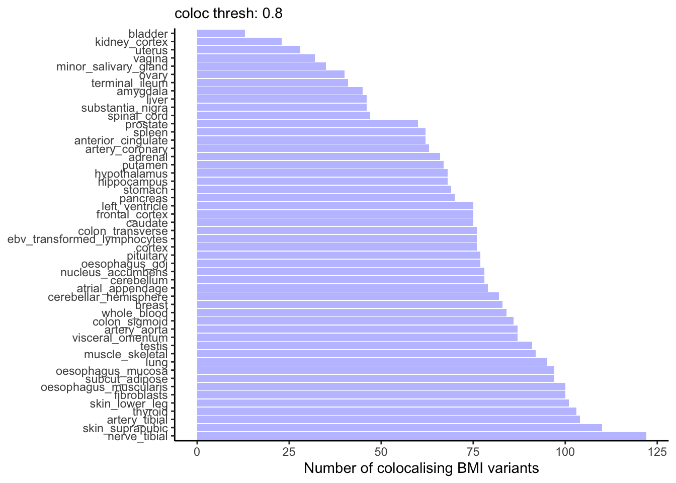
Determinants of colocalisation number
Does the number of colocalising variants, and/or the mean PPH4 value (across all BMI variants) for each tissue, depend on eQTL sample size? Yes, this appears to be important.
ggplot(coloc_counts, aes(x = mean_sample_n, y = num_coloc_pph4, color = mean_pph4, size = num_coloc_genes)) +
  geom_point() +
  geom_text_repel(aes(label = tissue), size = 2, color="black", max.overlaps = Inf) +
  scale_color_viridis_c(option="mako") +
  theme_classic() +
  labs(subtitle = paste("coloc thresh:", coloc_thresh),
       color = "Mean PPH4",
       size = "No. coloc genes",
       y = "No. colocalising BMI variants",
       x = "Sample size")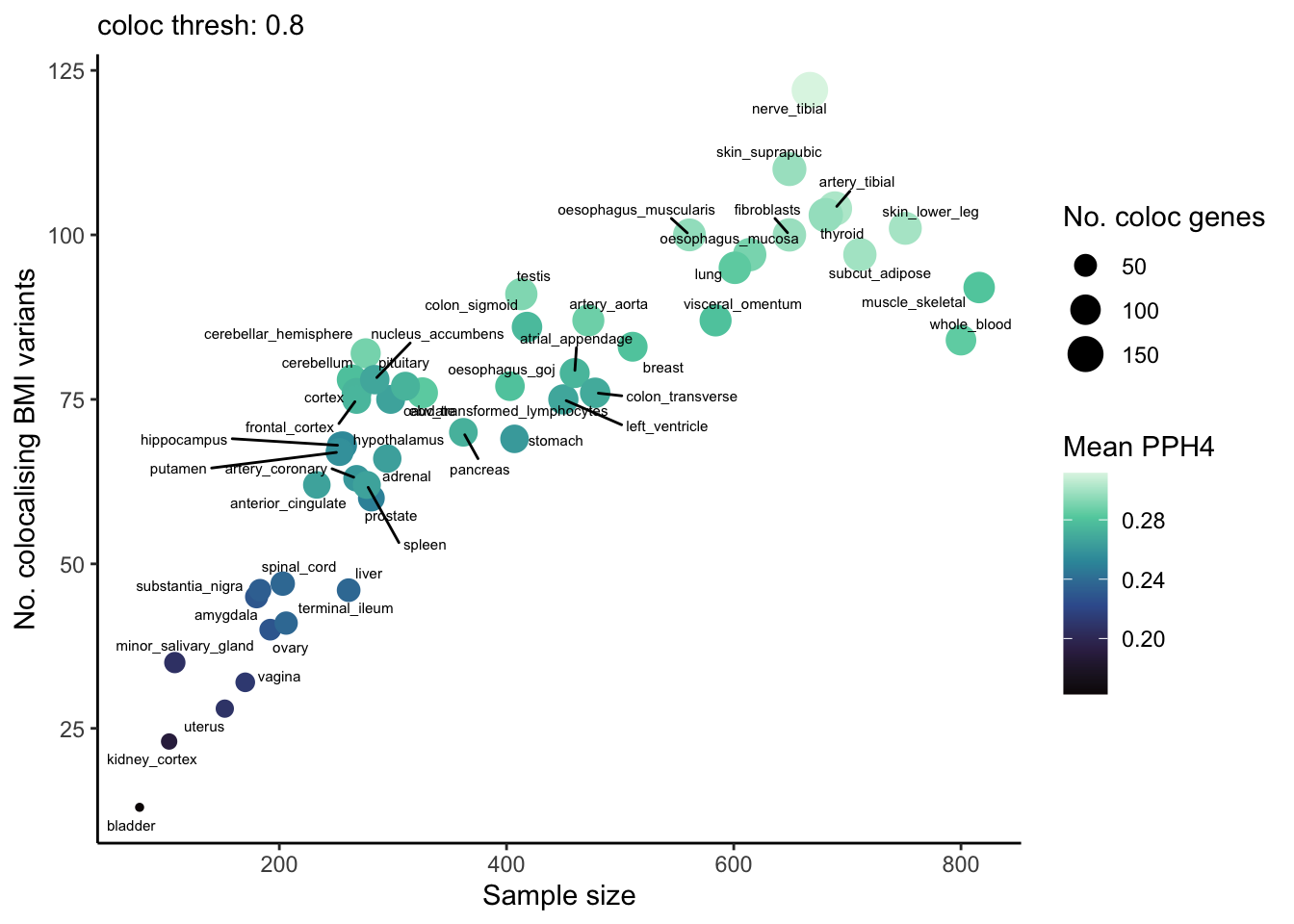
Effect of number of colocalising loci on MVMR result - 1
Simple simulation - hows does the number of variants used as an instrument effect the MVMR result. Let’s hold constant the number of colocalising variants in tissue 1 (set to median: 76) and then vary the number of variants in tissue 2. For now, let’s hold the PPH4 weighting for colocalising variants at constant 0.9 and the for the non-colocalising tissue variants something low, like 0.2. We see that the MVMR estimate flips when the second tissue has more variants than the first. The tissue with higher numbers of variants has the large MVMR estimate.
num_loci <- expand.grid(num_t1  = round(median(coloc_counts$num_coloc_pph4)),
                        num_t2  = seq(min(coloc_counts$num_coloc_pph4), max(coloc_counts$num_coloc_pph4)),
                        pph4_hi = 0.9,
                        pph4_lo = 0.2) |> as.data.table()

unique_num_loci <- sort(unique(c(num_loci$num_t1, num_loci$num_t2)))
unique_num_loci <- setNames(unique_num_loci, as.character(unique_num_loci))

loci_indicies <- lapply(unique_num_loci, function(num_l) {
  set.seed(123)
  sample(1:length(h_mvmr@snps), num_l, replace = FALSE)
})

mr_num_loci <- num_loci[, {
  h_tmp   <- copy(h_mvmr)
  t1_incides <- loci_indicies[[as.character(num_t1)]]
  t2_incides <- loci_indicies[[as.character(num_t2)]]
  h_tmp@index_snp <- ifelse(1:length(h_tmp@snps) %in% union(t1_incides, t2_incides), TRUE, FALSE)
  h_tmp@bx[t1_incides,1] <- h_tmp@bx[t1_incides,1] * pph4_hi
  h_tmp@bx[t2_incides,2] <- h_tmp@bx[t2_incides,2] * pph4_hi
  h_tmp@bx[setdiff(t2_incides, t1_incides),1] <- h_tmp@bx[setdiff(t2_incides, t1_incides),1] * pph4_lo
  h_tmp@bx[setdiff(t1_incides, t2_incides),2] <- h_tmp@bx[setdiff(t1_incides, t2_incides),2] * pph4_lo
  h_tmp@exposure <- c("Tissue 1", "Tissue 2")
  r <- run_mr(h_tmp, methods="mr_ivw")
}, by = .(num_t1, num_t2)]

ggplot(mr_num_loci[, `:=`(b_lb = b-b_se*1.96,
                          b_ub = b+b_se*1.96)],
       aes(x=num_t2, y=b, ymin=b_lb, ymax=b_ub, color=exposure)) +
  geom_errorbar(width=0.2, position = position_dodge(0.2)) +
  geom_point(position = position_dodge(0.2)) +
  theme_bw() +
  labs(y = "MVMR estimate (tpBMI vs HF)",
       x = "Number of tissue 2 loci",
       color = "Tissue",
       subtitle = paste0("Number of loci for tissue 1 fixed at ", num_loci$num_t1[1]))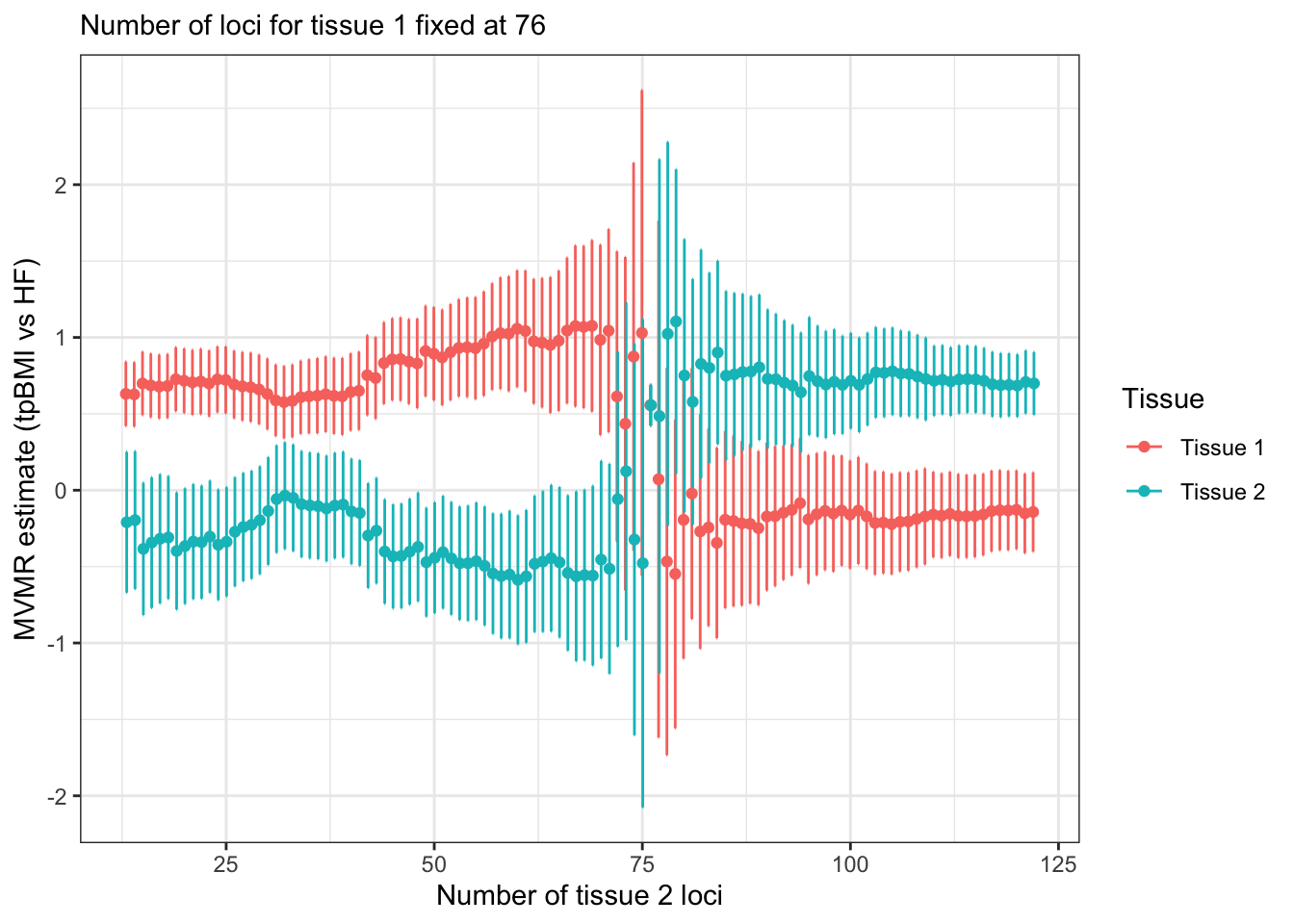
Effect of number of colocalising loci on MVMR result - 2
Now do the same but vary both the number of colocalising variants in tissue 1 and 2, and the percentage overlap of the instruments (grid search). We see that there has to be some difference in the number of colocalising loci and there needs to be some overlap of the loci in order to separate the MVMR results for each tissue.
num_loci <- expand.grid(num_t1  = seq(min(coloc_counts$num_coloc_pph4), max(coloc_counts$num_coloc_pph4), 50),
                        num_t2  = seq(min(coloc_counts$num_coloc_pph4), max(coloc_counts$num_coloc_pph4), 50),
                        overlap = seq(0, 1, 0.2),
                        seed    = 2000:2100,
                        pph4_hi = 0.9,
                        pph4_lo = 0.1) |> as.data.table()

library(future)
library(furrr)
plan(multisession)
mr_num_loci <- future_pmap_dfr(num_loci, function(num_t1, num_t2, overlap, seed, pph4_hi, pph4_lo) {

  h_tmp   <- copy(h_mvmr)

  # randomly sort the BMI SNP indices
  set.seed(seed)
  sram_idx <- sample.int(length(h_mvmr@snps))

  # indicies of the variants to use
  overlap_n <- round(min(num_t1, num_t2) * overlap)
  t1i       <- sram_idx[1:num_t1]
  t2i       <- sram_idx[(num_t1-overlap_n+1):(num_t2 + num_t1-overlap_n)]
  t12i      <- intersect(t1i, t2i)  # both tissues
  ut1i      <- setdiff(t1i, t12i)   # only tissue 1
  ut2i      <- setdiff(t2i, t12i)   # only tissue 2

  # which snps go into the instrument
  h_tmp@index_snp <- 1:length(h_mvmr@snps) %in% c(t12i, ut1i, ut2i)

  # weight tissue 1 betas
  h_tmp@bx[ut2i,1] <- h_tmp@bx[ut2i,1] * pph4_lo
  h_tmp@bx[t1i,1]  <- h_tmp@bx[t1i,1] * pph4_hi

  # weight tissue 2 betas
  h_tmp@bx[ut1i,2] <- h_tmp@bx[ut1i,2] * pph4_lo
  h_tmp@bx[t2i,2]  <- h_tmp@bx[t2i,2] * pph4_hi

  # naming
  h_tmp@exposure <- c("MV-beta tissue 1", "MV-beta tissue 2")

  # run mr
  r <- run_mr(h_tmp, methods="mr_ivw")

  r[, `:=`(num_t1   = num_t1,
           num_t2   = num_t2,
           num_diff = num_t1-num_t2,
           overlap  = overlap,
           seed     = seed,
           pph4_lo  = pph4_lo,
           pph4_hi  = pph4_hi)]

  return(r)
})


ggplot(mr_num_loci[, num_diff_lab := paste0("Delta~nSNP[T1-T2]:~ ", num_diff)],
       aes(x=as.factor(overlap), y=b, fill=exposure, color=num_t1)) +
  geom_hline(yintercept = 0.0, linetype="dashed", color="darkgray") +
  geom_violin(width=1, position= position_dodge(width = 0.5), color=NA) +
  scale_x_discrete(labels = function(x) scales::percent(as.numeric(x))) +
  theme_classic() +
  theme(legend.position = "top") +
  labs(x = "Instrument SNP overlap (% of smaller instrument)",
       y = "MVMR estimate",
       fill = "Tissue") +
  facet_wrap(~num_diff_lab,
             nrow = 1,
             labeller = label_parsed)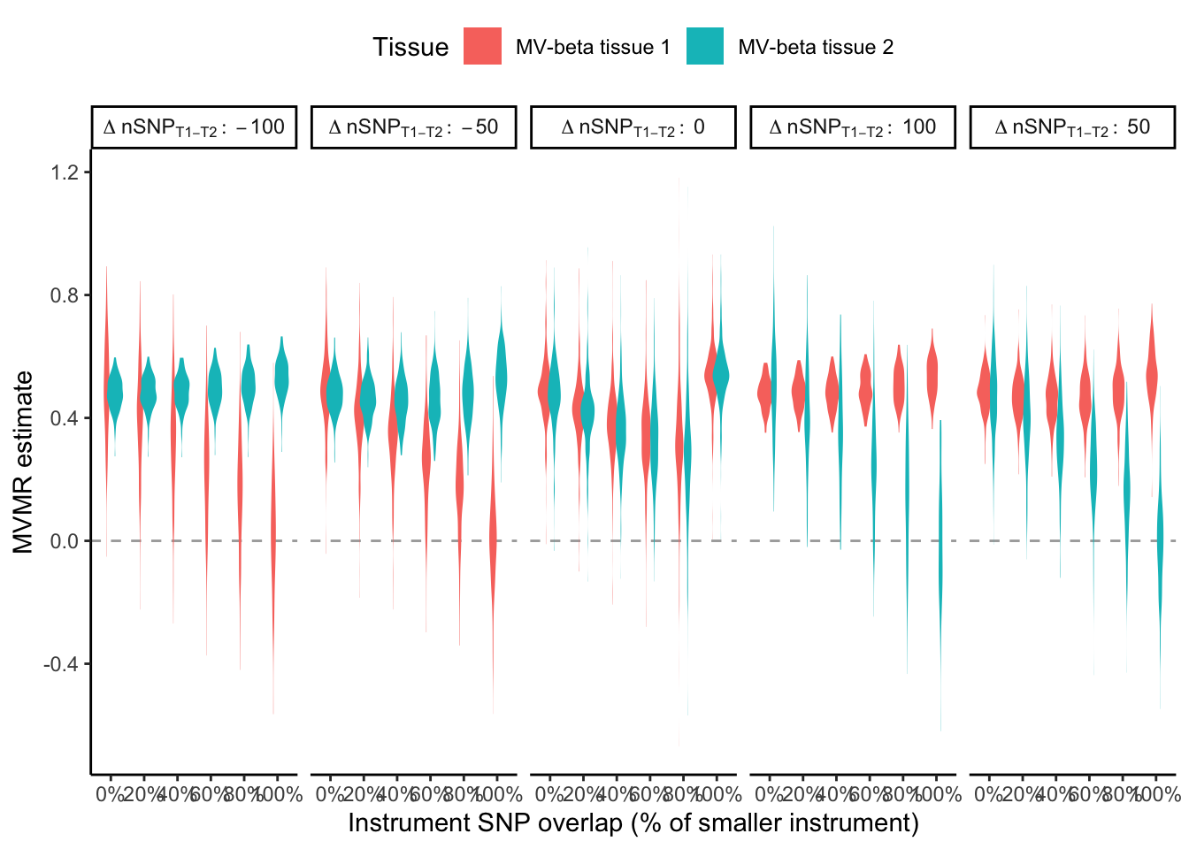
BMI:eQTL PPH4 distributions by tissue
Now lets look at the actual distributions of the PPH4 values in each tissue, since they are not fixed like in the above analyses. Take the maximum PPH4 from genes in close proximity to each variant, in each tissue and plot the distributions - these are the weights that would be used in the tissue-partitioned MR procedure.
num_tissues <- 6
tissues_subset <- levels(coloc_counts$tissue)[as.integer(seq(1, length(levels(coloc_counts$tissue)), length.out=num_tissues))]
coloc_subset <- coloc_results[locus_trait=="bmi" & trait.x=="bmi" & (trait.y %in% tissues_subset) & grepl("protein_coding", gene_type.y), .SD[which.max(pph4)], by=.(locus_index_rsid,trait.y)]

density <- coloc_subset[, {
  den <- density(pph4, n=1000)
  .(pph4 = scales::rescale(den$x, 0:1), prob = den$y)
}, by = c(tissue="trait.y")][, tissue := factor(tissue, levels = levels(coloc_counts$tissue))]

ggplot(density, aes(x=pph4, y=prob, color=tissue)) +
  theme_classic() +
  geom_line() +
  labs(y = "Density")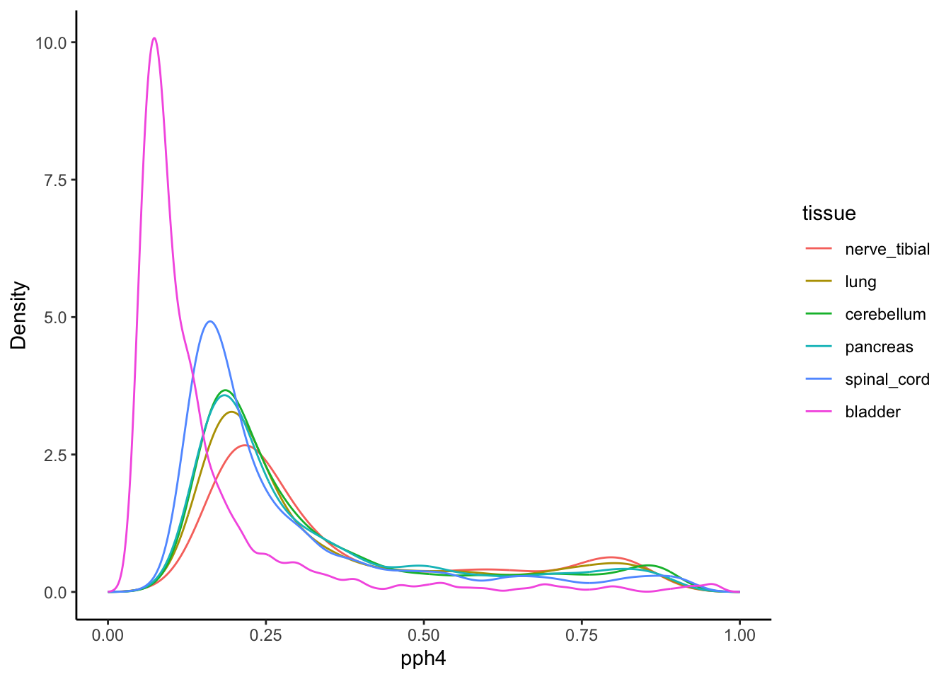
Use of these distributions in simulations
If we want ‘real-world’ PPH4 weights for use in simulations we can just sample from these density distributions. Here is a quick check to show that sampling from them replicates the shape.
tissues <- expand.grid(tissue = unique(density$tissue), stringsAsFactors = F) |> as.data.table()

set.seed(123)

res_sim_density <- tissues[, {
  .(sim_pph4 = sample(density[tissue==.BY$tissue, pph4], round(length(h_mvmr@bx[,1])/2), prob = density[tissue==.BY$tissue, prob], replace = TRUE))
}, by = .(tissue)]


ggplot(res_sim_density, aes(x=sim_pph4, color=tissue)) +
  theme_classic() +
  geom_density() +
  labs(y = "Simulated density",
       x = "Simulated PPH4",
       color = "Tissue")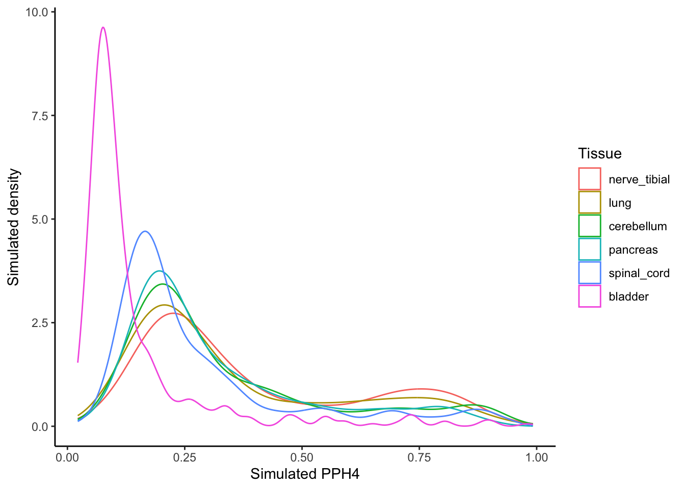
Effect different PPH4 weights
Weight the BMI betas by their respective maximum PPH4 value, see how this changes the relationship between the beta for BMI and beta for HF, dependent on which tissue is providing the betas. Tissues with greater or fewer colocalising variants affect push the betas up or down more, respectively. I hold one tissue constant (reference) to more easily appreciate how the other tissue’s colocalisation characteristics affect things.
ref_tissue   <- levels(density$tissue)[1]
tissue_pairs <- expand.grid(t1 = ref_tissue, t2 = unique(density$tissue), stringsAsFactors = F) |> as.data.table()

set.seed(123)
t1_pph4 <- sample(density[tissue==ref_tissue, pph4], length(h_mvmr@bx[,1]), prob = density[tissue==ref_tissue, prob], replace = TRUE)

res_weighted <- tissue_pairs[, {
  h_tmp <- h_mvmr
  t2_pph4 <- sample(density[tissue==.BY$t2, pph4], length(h_tmp@bx[,1]), prob = density[tissue==.BY$t2, prob], replace = TRUE)
  h_tmp@bx[,1] <- h_tmp@bx[,1] * t1_pph4
  h_tmp@bx[,2] <- h_tmp@bx[,2] * t2_pph4
  h_tmp@index_snp <- ifelse(t1_pph4>coloc_thresh | t2_pph4>coloc_thresh, TRUE, FALSE)
  .(tissue   = rep(c(paste0("Ref: ", ref_tissue),"Comparator"), each=sum(h_tmp@index_snp)),
    beta_bmi = c(h_tmp@bx[h_tmp@index_snp,1], h_tmp@bx[h_tmp@index_snp,2]),
    beta_hf  = rep(h_tmp@by[h_tmp@index_snp],2),
    mean_pph4_t1 = mean(t1_pph4[t1_pph4>coloc_thresh | t2_pph4>coloc_thresh]),
    mean_pph4_t2 = mean(t2_pph4[t1_pph4>coloc_thresh | t2_pph4>coloc_thresh]),
    rmse_pph4    = sqrt(mean((t1_pph4[t1_pph4>coloc_thresh | t2_pph4>coloc_thresh] - t2_pph4[t1_pph4>coloc_thresh | t2_pph4>coloc_thresh])^2))
   )
}, by = .(t1,t2)]
res_weighted[, t2 := factor(t2, levels = unique(t2[order(-mean_pph4_t1)]))]

ggplot(res_weighted, aes(x=beta_bmi, y=beta_hf, color=tissue)) +
  geom_point() +
  geom_text(data = unique(res_weighted[grepl("Ref", tissue)], by="t2"),
            aes(x = 0.0,
                y = -0.04,
                label = sprintf("Tis mPPH4=%.3f", mean_pph4_t2)),
            color="black", size=2) +
  geom_text(data = unique(res_weighted[!grepl("Ref", tissue)], by="t2"),
            aes(x = 0.0,
                y = -0.07,
                label = sprintf("Ref mPPH4=%.3f", mean_pph4_t1)),
            color="black", size=2) +
  geom_smooth(method="lm", se=F,fullrange = TRUE) +
  facet_wrap(~t2, labeller = labeller(t2 = function(x) gsub("_", " ", x))) +
  labs(subtitle = paste("coloc thresh:", coloc_thresh),
       y = "Heart failure beta",
       x = "BMI beta (PPH4-weighted)",
       color = "Tissue")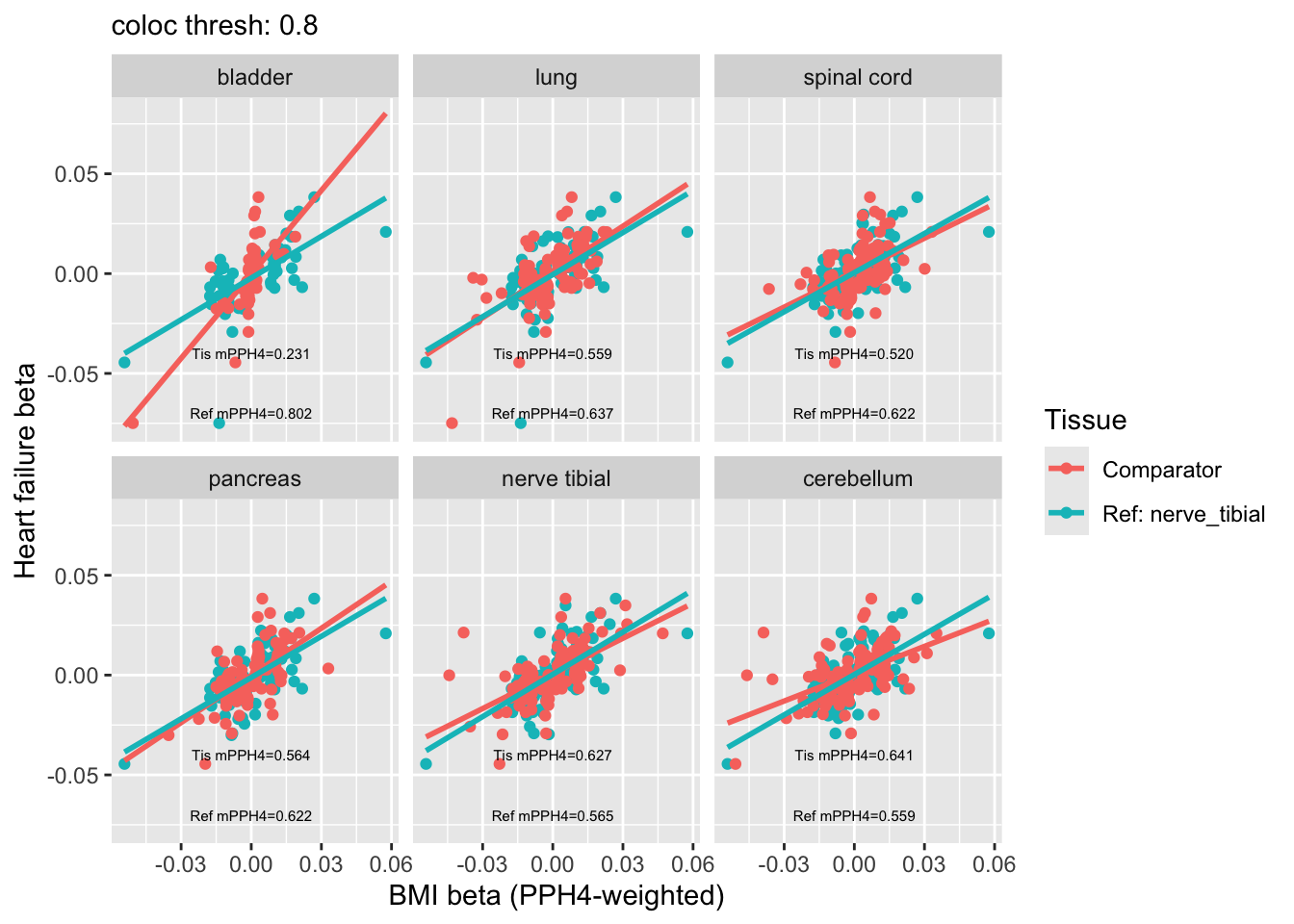
IVW regression by different PPH4 weighting distributions
Perform MVMR with the weighted BMI instruments. Lets look at varying the distributions that the PPH4 values are drawn from. Poorly colocalising tissues MVMR result is penalised against more highly colocalising tissues.
Function to weight betas and run MR
#' @title TPMR helper function
#' @param mrobj genepi.utils MR object (exposures BMI:BMI, outcome HF)
#' @param density data.table of PPH4 density distributions cols: tissue | pph4 | prob
#' @param ref character vector, tissues in density$tissue
#' @param comp character vector, tissues in density$tissue
#' @param coloc_thresh numeric 0-1
#' @param rep integer, number of replications (random sampling of BMI variants into instrument)
#' @returns data.table of MR results
#'
tpmr <- function(obj, ref, comp, coloc_thresh, rep = 1, density = NULL, pph4 = NULL) {

  # either density or actual PPH4 values
  stopifnot("Provide either denisty distributions or actual PPH4 values" =
              sum(sapply(list(density, pph4), is.null)) == 1)
  stopifnot("Replications must be 1 if using actual PPH4 values" = ifelse(rep > 1 & !is.null(pph4), F, T))

  # run the MR for each of the exposure combinations
  tissue_pairs <- expand.grid(t1 = as.character(ref),
                              t2 = as.character(comp),
                              seed = 2000:(2000+rep-1),
                              stringsAsFactors = F) |> as.data.table()

  library(future)
  library(furrr)
  plan(multisession)
  mr_weighted <- future_pmap_dfr(tissue_pairs, function(t1, t2, seed) {

    mrobj <- copy(obj)

    if (!is.null(density)) {

      # generate the PPH4 values randomly for the variants
      set.seed(seed)
      t1_pph4 <- sample(density[tissue==t1, pph4], length(mrobj@snps), prob = density[tissue==t1, prob], replace = TRUE)
      set.seed(seed+1)
      t2_pph4 <- sample(density[tissue==t2, pph4], length(mrobj@snps), prob = density[tissue==t2, prob], replace = TRUE)

    } else if(!is.null(pph4)) {

      chrpos <- data.table(chr = as.integer(mrobj@chr), bp = mrobj@bp, t1 = t1, t2 = t2)
      chrpos[pph4, t1.pph4 := i.pph4, on=c("chr"="chr","bp"="bp","t1"="tissue")]
      chrpos[pph4, t2.pph4 := i.pph4, on=c("chr"="chr","bp"="bp","t2"="tissue")]
      t1_pph4 <- chrpos$t1.pph4
      t2_pph4 <- chrpos$t2.pph4
      t1_pph4[is.na(t1_pph4)] <- 0
      t2_pph4[is.na(t2_pph4)] <- 0

    }

    # based on the distribution of PPH4, which SNPs are included
    include <- ifelse(t1_pph4 > coloc_thresh | t2_pph4 > coloc_thresh, TRUE, FALSE)

    # update the MR object, turn off the excluded snps (@index_snp slot)
    mrobj@bx[,1]      <- mrobj@bx[,1] * t1_pph4
    mrobj@bx[,2]      <- mrobj@bx[,2] * t2_pph4
    mrobj@index_snp   <- include
    mrobj@exposure[1] <- ifelse(length(ref)==1, paste0("Ref: ", ref_tissue), "Tissue 1")
    mrobj@exposure[2] <- ifelse(length(ref)==1, "Comparator", "Tissue 2")

    # run the MR
    r <- run_mr(mrobj, methods="mr_ivw")

    # add info about the instrument used
    r[, `:=`(t1             = t1,
             t2             = t2,
             seed           = seed,
             n_sig_snps     = c(sum(t1_pph4 > coloc_thresh), sum(t2_pph4 > coloc_thresh)),
             n_overlap_snps = sum(t1_pph4 > coloc_thresh & t2_pph4 > coloc_thresh),
             pct_t1_overlap = sum(t1_pph4 > coloc_thresh & t2_pph4 > coloc_thresh) / length(t1_pph4),
             mean_pph4_t1   = mean(t1_pph4[include]),
             mean_pph4_t2   = mean(t2_pph4[include]),
             rmse_pph4      = sqrt(mean((t1_pph4[include] - t2_pph4[include])^2)),
             rmse_wbeta     = sqrt(mean((mrobj@bx[,1] - mrobj@bx[,2])^2)))]
    r[, c("overdispersion", "n_pc", "n_hunted", "slopehunter_pi", "slopehunter_ent") := NULL]

  })

  return(mr_weighted)
}
Different PPH4 distributions against each other
# run TPMR
mr_weighted <- tpmr(obj=h_mvmr, density=density,
                    ref= unique(density$tissue),
                    comp=unique(density$tissue),
                    coloc_thresh=0.8,
                    rep = 100)

# reorder for plotting
mr_weighted[, mean_pph4_t1_lab := round(mean(mean_pph4_t1),2), by=.(t1)]
mr_weighted[, mean_pph4_t2_lab := round(mean(mean_pph4_t2),2), by=.(t2)]
mr_weighted[, mean_n_sig_snps := round(mean(mean_pph4_t2),0), by=.(t1,t2)]

ggplot(mr_weighted,
       aes(x=as.factor(mean_pph4_t2_lab), y=b, color=exposure)) +
  geom_boxplot() +
  theme_bw() +
  labs(y = "MVMR estimate", x = "T2 mean PPH4", color = "Tissue") +
  facet_wrap(~ as.factor(mean_pph4_t1_lab),
             labeller = labeller(`as.factor(mean_pph4_t1_lab)`=function(x) paste0("T1 mean PPH4: ",x)))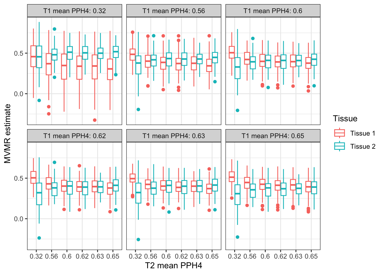
ggplot(mr_weighted[, .(b=mean(b)), by=.(t1,t2,exposure)][, .(b_diff=b[1]-b[2]), by=.(t1,t2)],
       aes(y=t1, x=t2, fill=b_diff)) +
  geom_tile() +
  scale_fill_gradient2() +
  theme(axis.text.x  = element_text(angle=45, hjust=1)) +
  labs(y = "Tissue 1", x = "Tissue 2", fill = "T1-T2 beta diff")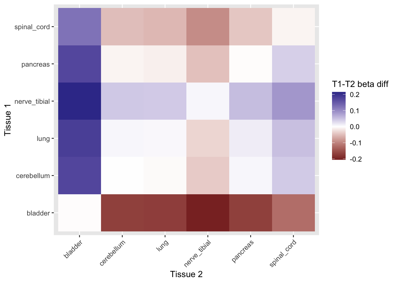
All tissue pairs MR (actual PPH4 values)
Now let’s use the real data and do the all GTEx tissue against all other GTEx tissues. The poorly colocalising tissues have lower MVMR estimates against more highly coloclising tissues.
tissue_pph4_vals <- coloc_results[locus_trait=="bmi" &
                                    trait.x=="bmi" &
                                    gene_type.y=="protein_coding",
                                  .SD[which.max(pph4)],
                                  by=.(locus_index_rsid, tissue=trait.y),
                                  .SDcols=c("chr", "bp", "pph4")]
tissue_pph4_vals <- tidyr::complete(tissue_pph4_vals, locus_index_rsid, tissue) |> as.data.table()

mr_actual <- tpmr(obj=h_mvmr, pph4=tissue_pph4_vals,
                  ref= unique(tissue_pph4_vals$tissue),
                  comp=unique(tissue_pph4_vals$tissue),
                  coloc_thresh=0.8)

ggplot((mr_actual
        [coloc_counts, t1_n := i.mean_sample_n, on=c("t1"="tissue")]
        [coloc_counts, t2_n := i.mean_sample_n, on=c("t2"="tissue")]
        [, `:=`(b_diff     = b[exposure=="Tissue 1"]-b[exposure=="Tissue 2"],
                snp_diff   = n_sig_snps[exposure=="Tissue 1"]-n_sig_snps[exposure=="Tissue 2"],
                pph4_diff  = mean_pph4_t1-mean_pph4_t2,
                nsamp_diff = t1_n - t2_n), by=.(t1,t2)]
        [, `:=`(t1 = factor(t1, levels = unique(t1[order(-b_diff)])),
                t2 = factor(t2, levels = unique(t1[order(-b_diff)])))]),
       aes(y=t1, x=t2, fill=b_diff)) +
  geom_tile() +
  scale_fill_gradient2() +
  theme(axis.text.x  = element_text(angle=45, hjust=1)) +
  labs(y = "Tissue 1", x = "Tissue 2", fill = "T1-T2 beta diff")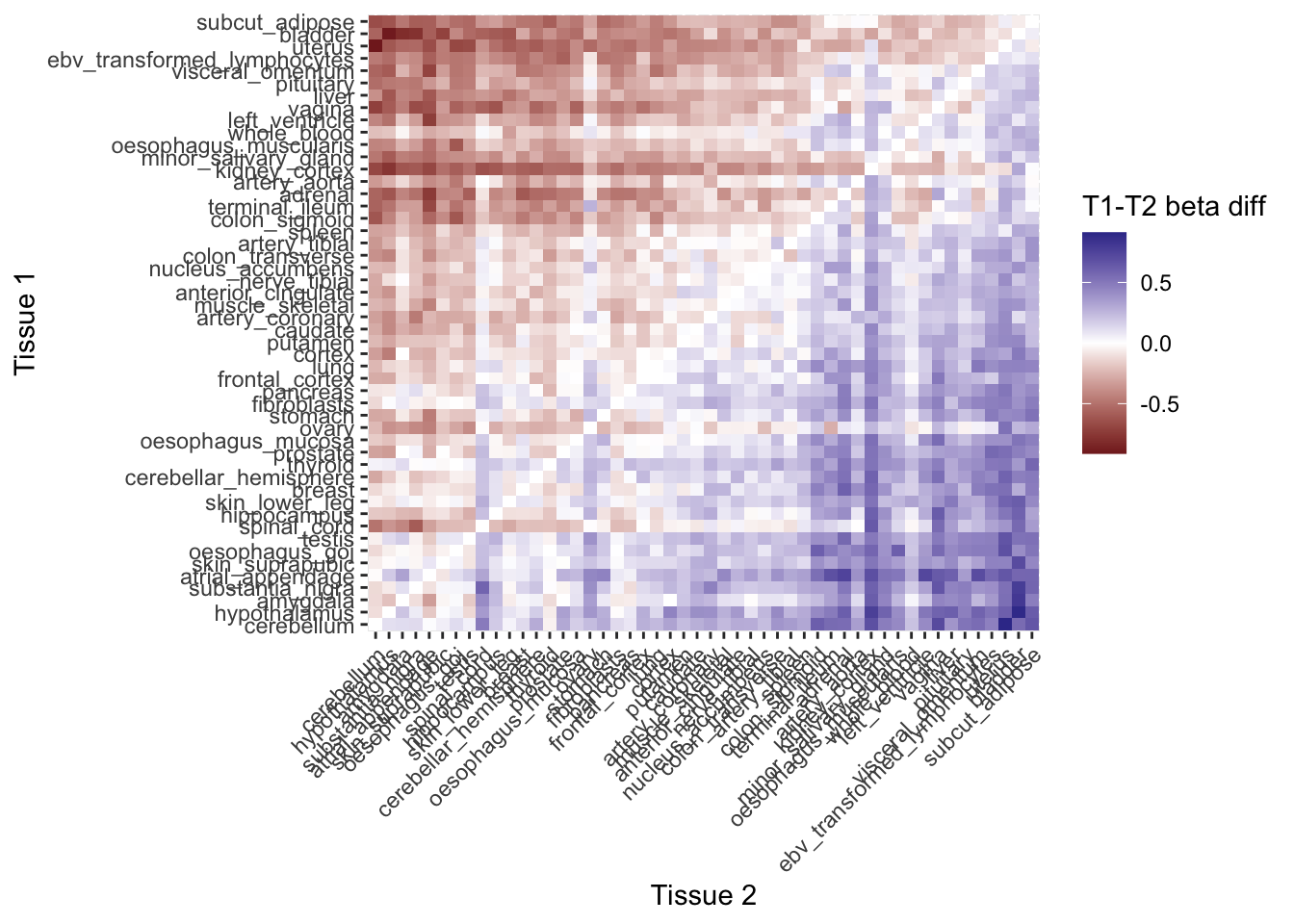
MVMR estimates depend on difference in instrument size (which also depends on difference in sample size)
Plot the different between MVMR estimates from a the 2-exposure MVMR procedure above - i.e. how separated are the effects attributed to each tissue. Is the magnitude of the separation related to the relative number of SNPs in each instrument, and does this depend on the sample size.
t1_highlight <- c("cortex", "frontal_cortex", "hippocampus", "hypothalamus")
t2_highlight <- c("subcut_adipose")
ggplot((mr_actual
        [coloc_counts, t1_n := i.mean_sample_n, on=c("t1"="tissue")]
        [coloc_counts, t2_n := i.mean_sample_n, on=c("t2"="tissue")]
        [, `:=`(b_diff     = b[exposure=="Tissue 1"]-b[exposure=="Tissue 2"],
                snp_diff   = n_sig_snps[exposure=="Tissue 1"]-n_sig_snps[exposure=="Tissue 2"],
                pph4_diff  = mean_pph4_t1-mean_pph4_t2,
                nsamp_diff = t1_n - t2_n), by=.(t1,t2)]
       ),
       aes(y=b_diff, x=snp_diff, color=nsamp_diff)) +
  geom_hline(yintercept = 0.0, linetype="dotted", color="grey") +
  geom_vline(xintercept = 0.0, linetype="dotted", color="grey") +
  geom_point(alpha=0.3) +
  geom_label_repel(data = unique(mr_actual[t1 %in% t1_highlight & t2 %in% t2_highlight][, lab := paste0(t1,"/",t2)], by="lab"), aes(label=lab), max.overlaps=Inf, nudge_y=0.5, color="black") +
  scale_color_viridis_c(option="magma") +
  geom_smooth(method="lm", se=FALSE, color="red") +
  theme_classic2() +
  theme(legend.position = "top") +
  labs(y = expression(Delta[T1-T2]~MVMR~estimate),
       x = expression(Delta[T1-T2]~No.~coloc~SNPs),
       color = expression(Delta[T1-T2]~Tissue~sample~size))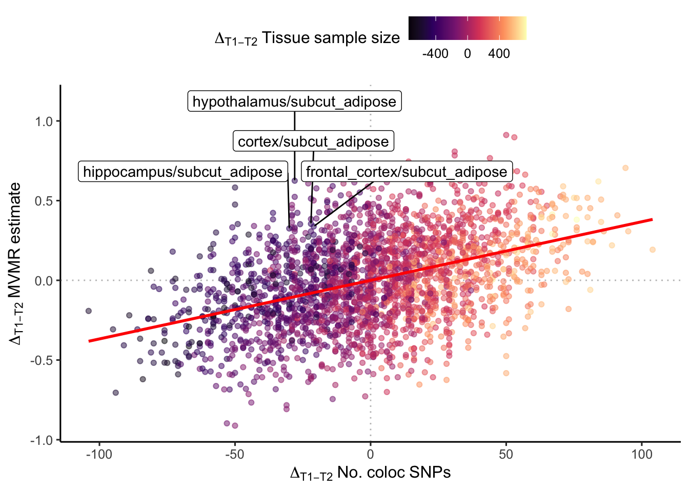
Interpretation so far
Is the MVMR estimate mostly related to the difference in the relative number of colocalising SNPs in tissue A vs. tissue B? The tissue with fewer colocalising SNPs may be overpowered in the MVMR by the tissue with a greater number of colocalising SNPs, since number of colocalising SNPs is related to sample size of the eQTL dataset, is the MVMR estimate just a function of sample size? We not clearly, as despite the trend there are numerous tissues which show the reverse pattern - e.g. brain tissues where the sample size and number of colocalising loci is actually less than for subcutaneous adipose tissue, yet the MVMR result yeilds a larger contribution from the brain tissue instrument (i.e. the points live in the North-West quantrant of the plot above). Let’s look at why this happens.
Brain vs adipose tissue
Lets break down the characteristics of the brain and adipose tissue-partitioned BMI instruments.
Number of colocalising loci
ggplot((coloc_counts
        [tissue %in% c(t1_highlight, t2_highlight)]
        [, tissue_class := ifelse(tissue %in% t1_highlight, "Brain", "Adipose")]
        ), aes(x = tissue, y = `num_coloc_pph4`, fill = tissue_class)) +
  theme_classic2() +
  geom_col(alpha = 0.5) +
  labs(subtitle = paste("coloc thresh:", coloc_thresh),
       y = "Number of colocalising BMI variants") +
  theme(axis.title.x = element_blank(),
        axis.text.x = element_text(angle=45, hjust=1)) +
  guides(fill = "none") +
  facet_wrap(~tissue_class, scales = "free_x")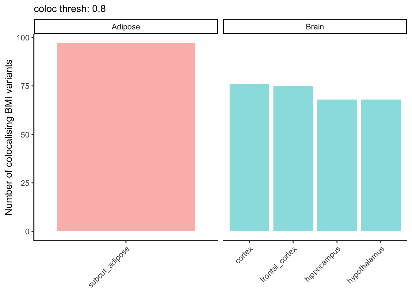
Distribution of PPH4
brain_adip_coloc <- coloc_results[locus_trait=="bmi" & trait.x=="bmi" & (trait.y %in% c(t1_highlight,t2_highlight)) & grepl("protein_coding", gene_type.y), .SD[which.max(pph4)], by=.(locus_index_rsid,trait.y)]
bmi_gwas_data <- as.data.table(h_mvmr)[, chr:= as.integer(chr)]
brain_adip_coloc[bmi_gwas_data, `:=`(bmi_beta = i.bx, weighted_bmi_beta = pph4*i.bx), on=.(chr,bp)]

ggplot(brain_adip_coloc, aes(x=pph4, color=trait.y)) +
  theme_classic() +
  geom_density() +
  labs(y = "Density", x = "PPH4", color="Tissue")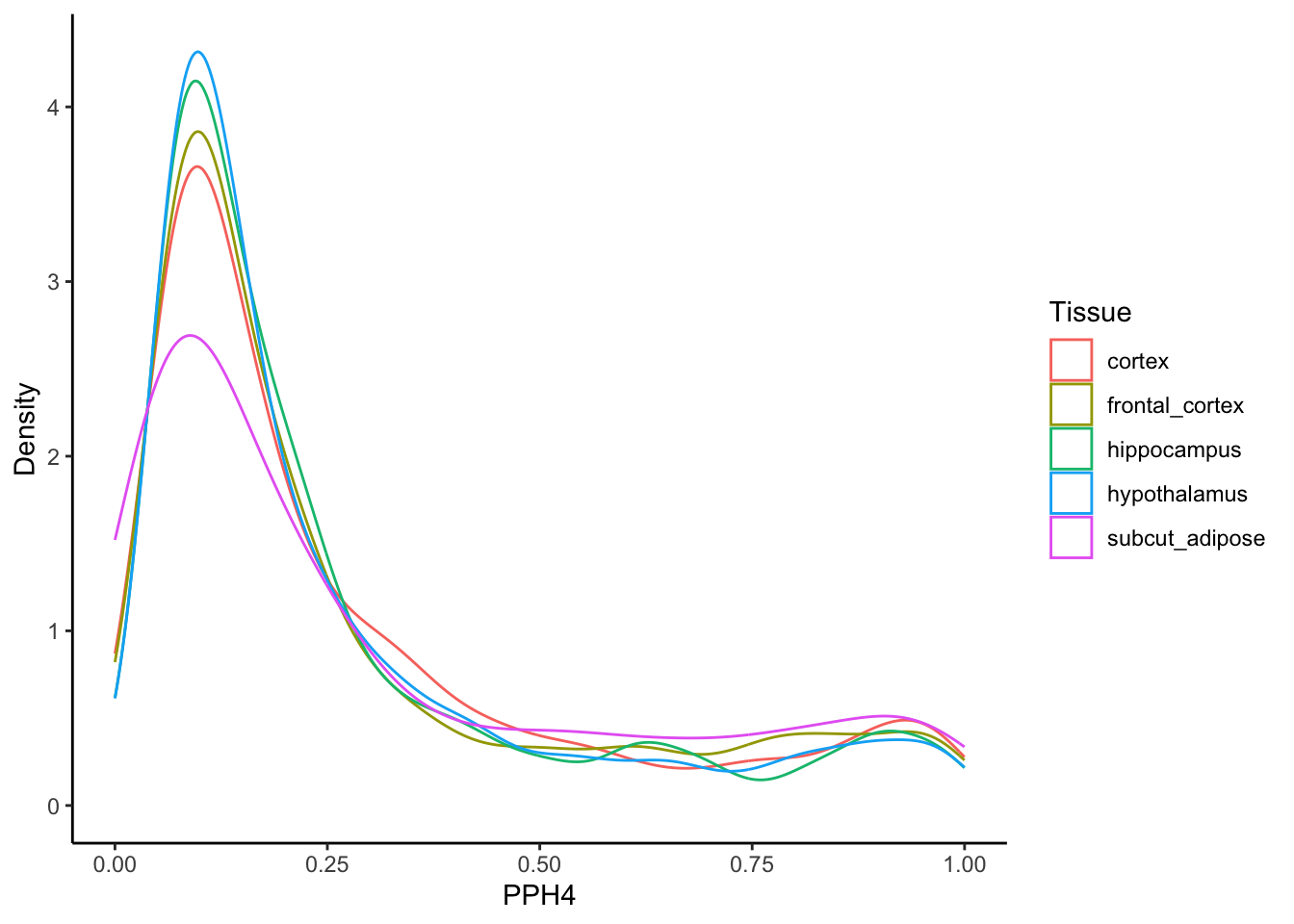
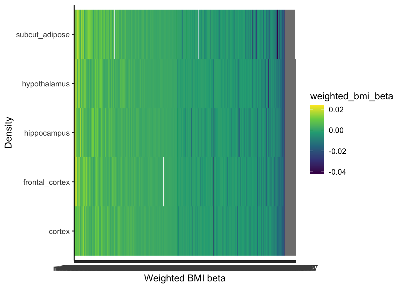
Distribution of weighted BMI betas (all)
ggplot(brain_adip_coloc[, locus_index_rsid:=factor(locus_index_rsid, levels=unique(locus_index_rsid[order(-weighted_bmi_beta)]))],
       aes(x=locus_index_rsid, y=trait.y, fill=weighted_bmi_beta)) +
  theme_classic2() +
  geom_tile() +
  scale_fill_viridis_c() +
  labs(y = "Density", x = "Weighted BMI beta", color="Tissue")